Advancing Statistical Literacy in Eye Care: A Series for Enhanced Clinical Decision-Making
Part 2: Statistical Testing in Eye and Vision Research – Principles and PracticesPurpose: To enhance statistical literacy in eye and vision Research through practical guidance on hypothesis testing, test selection, and interpreting inferential statistics. The goal is to reduce common analytical errors and support more clinically meaningful conclusions in ophthalmic studies.
Material and Methods: A narrative literature review was conducted using PubMed, Scopus, and Web of Science to identify best practices in hypothesis testing, error control, and test selection relevant to clinical research in ophthalmology
and optometry. Simulated datasets, based on real-world clinical scenarios, were generated in Python to illustrate core concepts. Worked examples demonstrate the Impact of sample size, data distribution, and error type on statistical
conclusions.
Results: Common misinterpretations of p-values and frequent misuse of statistical tests were identified. The review explains how reducing the significance level (α) increases Type II error risk unless the sample size is increased. A structured decision framework was developed to aid the choice between parametric and non-parametric tests, including when assumptions are violated. Simulations and clinical examples demonstrate how effect size, variability, and multiple testing adjustments affect results.
Conclusion: Statistical missteps in eye research often arise from poor test selection, inadequate power, or overreliance on p-values without context. This article advocates for the use of confidence intervals, effect sizes, and ransparent
reporting to enhance the credibility of research findings. Following structured analytic frameworks and established reporting guidelines (e. g. CONSORT, STROBE) helps ensure that statistical conclusions align with clinical relevance, ultimately supporting better patient care and more trustworthy research outcomes.
Introduction
Inferential statistics underpin evidence-based clinical Research by allowing conclusions to be drawn about populations from sample data. In eye and vision research (EVR), the appropriate selection and application of statistical Tests are essential for ensuring that study findings are valid and clinically meaningful. Despite widespread statistical education, persistent data analysis errors have been documented across biomedical literature.1 In ophthalmology, recurring issues include incorrect units of analysis, improper handling of multiple comparisons, and misinterpretation of results.2 These are not trivial mistakes; they can lead to flawed conclusions and potentially harmful clinical decisions, resulting in wasted resources and diminished research impact.3 Enhancing statistical literacy among clinicians and researchers is critical to
reducing avoidable errors in eye and vision studies.
Building on Part 1 4, this series (Part 2) emphasises inferential statistics, focusing on hypothesis testing and selecting the appropriate test for various study designs and data types. Part 1 introduced foundational concepts, including data types (nominal, ordinal, interval, ratio), data preparation techniques, and the importance of descriptive statistics and data visualisation for understanding sample characteristics. This second instalment builds directly on that foundation by addressing persistent shortcomings in statistical practice. For example, ophthalmic trials have frequently demonstrated low statistical power and elevated risks of Type II errors (false negatives).5 Inadequate attention to test assumptions and power calculations may lead to the missed detection of clinically relevant effects or the reporting of spurious results due to uncontrolled multiple comparisons. The clinical consequences of such errors are substantial. Day-to-day decisions in eye care, such as whether to adopt a new therapy or interpret a diagnostic test, depend on reliable evidence. Inappropriate test selection or misinterpretation of results undermines that reliability. Conversely, robust statistical methods strengthen the evidence base, enabling the detection of meaningful effects and guiding practice with greater confidence. Well-conducted ophthalmic trials have demonstrated how rigorous analysis can inform treatment guidelines and enhance Patient care.5,6,7 Strengthening statistical literacy among eye care professionals is crucial for enhancing the quality of Research and improving the effectiveness of clinical decision-making.
Methods
The methods used in this article have been described in Part 1 of this series.4 In brief, a narrative literature review was conducted using PubMed, Scopus, and Web of Science databases to identify best practices in statistical testing for EVR. Simulated datasets were created in Python to illustrate core concepts, reflecting typical clinical scenarios in ophthalmology, optometry, and vision science. All data are synthetic and intended solely for educational use. To reinforce key principles, supplementary materials include worked examples.
Hypothesis testing principles in eye & vision research
Most clinical research begins with a question: for example, “Does treatment A improve (e.g. visual acuity) more than treatment B in patients with (e.g. age-related macular degeneration)?” Hypothesis testing provides a formal framework to answer such questions with quantitative evidence. The basic principle is to pose two opposing hypotheses and use sample data to determine which is better supported.
- Null Hypothesis (H₀): Generally, a statement that there is no difference between groups or no effect of an intervention. It posits that any observed difference in outcomes is due to chance. For our example, H₀ might state, “There is no significant difference in mean visual acuity improvement between treatment A and treatment B.”
- Alternative Hypothesis (H₁ or Hα): Directly following the null hypothesis is the alternative hypothesis, which is the statement of an effect or difference – what the researcher hopes or expects to find. In the example, H₁ might be “Treatment A leads to greater mean improvement in visual acuity than treatment B.”
Phrasing the null and alternative hypotheses correctly is one of the most crucial steps in designing and conducting research, as they define every subsequent step. Data are collected once the hypotheses are described, and an appropriate statistical test is selected based on the study design and data characteristics. The analysis yields a test statistic and a corresponding p-value. The p-value represents the probability of obtaining data as extreme as (or more extreme than) what was observed, assuming the null hypothesis is true.8,9 It is a measure of compatibility between the observed data and the null hypothesis, not the probability that the null hypothesis is true.
A p-value of 0.03 means that if there were truly no difference between the treatments, there would be a 3 % chance of observing a result as extreme as the one found, purely due to random variation. This does not mean there is a 97 % chance that the alternative hypothesis is correct. That is a common misinterpretation. The p-value provides information about the null hypothesis, not about the alternative. It reflects how compatible the observed data are with the assumption that there is no effect or difference. Statistical tests do not directly prove the null hypothesis is false. Instead, if the data are unlikely under the assumption that the null hypothesis is true, this is considered evidence against the null hypothesis and in favour of the alternative.
The researcher must determine, based on professional judgment, risk assessment, and review of relevant literature, how much uncertainty is acceptable in a given study. This pre-specified threshold for uncertainty is known as the significance level, often denoted by alpha (α). It defines the maximum probability of making a Type I error, incorrectly rejecting the null hypothesis when it is actually true. A significance level (denoted α or Type I error) is set before data analysis, typically at 0.05, to guide decision-making. If p < α, the null hypothesis is rejected, and the result is said to be statistically significant.
If p ≥ α, the null hypothesis is not rejected. However, failure to reject H₀ does not imply it is true; it may simply reflect insufficient evidence, often due to small sample size or high variability. The balance between having sufficient evidence to detect a true effect and managing error rates is addressed during the study design phase through a priori power calculations to determine an adequate sample size.
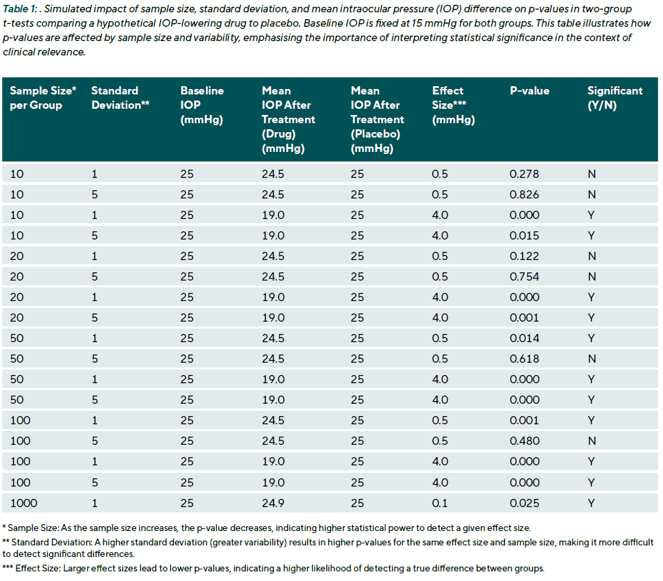
In EVR, where numerous biological and measurement factors may influence outcomes such as visual acuity, IOP, or retinal thickness, interpreting p-values in isolation can be misleading. A statistically significant result does not necessarily imply clinical significance. For example, a mean IOP reduction of 0.5 mmHg with a p-value of 0.04 may be statistically significant but clinically negligible. Conversely, a p-value just above 0.05, say, 0.06, should not automatically be dismissed, especially if the effect size is meaningful and consistent with prior evidence. Moreover, p-values are sensitive to sample size. Extensive studies can produce very small p-values for trivial effects, while small studies may yield non-significant p-values despite clinically important differences (Table 1). Therefore, effect sizes and confidence intervals should always accompany p-values to provide context.
The confidence interval indicates the range within which the true effect is likely to lie, and its width reflects the precision of the estimate. While p-values play a central role in hypothesis testing, they should not be treated as the sole arbiter of truth. Interpreting them requires careful consideration of the study design, effect size, confidence intervals, and the clinical context. Overreliance on arbitrary thresholds (e.g., p < 0.05) without proper context risks drawing misleading conclusions, (Table 1).
Clinical example 1: To illustrate the interpretation of a p-value, consider a clinical trial comparing a new eyedrop to standard treatment for lowering IOP. After four weeks, the mean IOP reduction is 3.0 mmHg in the treatment group (range: 0.5 to 6.0 mmHg) and 2.0 mmHg in the control group (range: –0.5 to 5.5 mmHg). A two-sample t-test yields p = 0.04. This suggests that, assuming no true difference exists between treatments (i.e., the null hypothesis is true), there is a 4 % chance of observing a difference of 1.0 mmHg or more purely by chance. The result is statistically significant at the conventional threshold of α = 0.05. While the difference is statistically significant, this does not guarantee clinical relevance. The observed ranges show natural variation within each group, which occurs even when treatments are similarly effective.
Type I and Type II errors
In hypothesis testing, there are two types of errors that can occur in the decision-making process, both of which have special relevance in clinical research:
- Type I Error (False Positive): This occurs when we reject the null hypothesis when it is actually true. In essence, this is a „false alarm,“ concluding there is a difference or an effect when, in reality, there is none. The probability of making a Type I error is determined by the significance level, α. For example, with α = 0.05, there is a 5 % risk of „discovering“ a difference that isn‘t truly there. In EVR, a
Type I error could mean believing a new drug improves visual acuity when it has no effect, potentially leading to the adoption of an ineffective treatment. - Type II Error (False Negative): This occurs when we fail to reject the null hypothesis when it is actually false. In other words, this is a „missed opportunity“ - failing to detect a real effect or difference. The probability of a Type II error is denoted by β. The statistical power of a test, which is the probability of correctly detecting a true effect, is calculated as (1 − β). In EVR, a Type II error could mean overlooking a real benefit of a new glaucoma therapy because the study was too small or the data too variable. Historically, less attention was given to controlling Type II errors, but this is changing, as underpowered studies have significant ethical and scientific implications. For example, a review of ophthalmology trials found that a large portion had a high risk of Type II errors, meaning real, clinically relevant effects could easily have been missed due to insufficient sample sizes.5
The researcher must balance two types of errors in statistical testing: false positives (Type I errors) and false negatives (Type II errors). This trade-off can be illustrated using the image of a bowl filled with sand, where the sand represents the total amount of potential error. Removing sand from one side of the bowl simply results in a mound forming on the other side. The total amount of error remains the same unless the size of the bowl is increased. In statistical terms, reducing the significance level (α) to lower the risk of false positives usually
increases the risk of false negatives (denoted by β), unless the sample size is increased. To manage this balance, researchers use study design strategies, including formal sample size calculations, to ensure the study has adequate power. Power refers to the probability of correctly detecting a true effect, and typical targets are 80 % or 90 %, which correspond to β values of 0.2 or 0.1, respectively. For example, when designing an ophthalmic clinical trial, the researcher calculates the required number of participants needed to detect a clinically meaningful difference, such as a five-letter improvement in visual acuity, with high power at the selected α level.
One-Tailed versus Two-Tailed Tests
Another consideration in hypothesis testing is whether to use a two-tailed (two-sided) or one-tailed test. A two-tailed test assesses for any difference in either direction, while a one-tailed test only examines a difference in a pre-specified direction. For example, when evaluating a new myopia control lens against a standard lens, a two-tailed H₁ might be: “There is a difference in mean myopic progression between lenses,” capturing both slower and faster progression. A one-tailed H₁ might state: “The new lens slows myopia progression more than the standard lens,” excluding the possibility of a negative effect. Although one-tailed tests offer greater power to detect an effect in the specified direction (since the entire α is allocated to one tail), they carry a substantial limitation: they ignore effects in the opposite direction, which may be clinically important or harmful. In the above example, if the new lens actually worsens progression, a one-tailed test focused
only on improvement would fail to detect it.
For this reason, two-tailed tests are standard in clinical research.10 The small loss in power is outweighed by the ethical and scientific importance of being open to detecting unexpected harm. Most peer-reviewed journals discourage or reject the use of one-tailed tests unless a very strong justification is provided, typically only when an effect in the opposite direction is truly impossible or irrelevant, which is rare in medical research.
Two-tailed tests are almost always preferred in eye and vision research. They protect against unanticipated harm and align with the principles of ethical clinical investigation. One-tailed tests should be reserved for exceptional cases with clear, pre-defined justification.
Clinical example 2: A clinical trial comparing a new retinal implant designed to restore vision in patients with advanced photoreceptor degeneration to standard care. The primary outcome is a functional visual score. The researchers hypothesise improvement with the implant. If they used a one-tailed test (α = 0.05, one-tailed), they might achieve significance with a smaller sample size if the implant is effective. However, if the implant unexpectedly caused some damage, leading to worse scores, a one-tailed test focused only on improvement would not register this decline as statistically significant, even if it was large. A two-tailed test (α = 0.05 split into 0.025 in each tail) would require more data to support improvement, but it would also flag a significant deterioration.
Parametric vs non-parametric tests: Assumptions and decision framework
Choosing the right statistical test depends on the type of data and whether certain assumptions are met. Broadly, statistical tests can be classified as parametric or non-parametric (distribution-free). Parametric tests assume that the data follow a specific distribution (typically a normal distribution for continuous data) and utilise model parameters, such as means and standard deviations. Non-parametric tests make
fewer assumptions about the data’s distribution and often rely on the rank-ordering of the data rather than the raw values. Both tests are widely used in EVR, and each has its place. Understanding when to use a parametric vs a non-parametric test is essential for valid analysis.
Parametric tests and their assumptions
Parametric tests are typically applied to continuous, approximately normally distributed data. Common assumptions include:
- Normality: The data should follow a normal distribution. This can be tested using normality tests, such as the Shapiro-Wilk Test.
- Homoscedasticity: The variances across comparison groups should be equal. This can be assessed using Levene‘s Test, which checks for equal variances among the different groups.
- Independence: The observations should not be correlated. This is typically ensured by the study design (e.g., recruiting separate individuals for each group) rather than a formal statistical test. For non-independent data, such as measurements from two eyes of the same person or repeated measures over time, specific analytical methods that account for the correlation must be used.
These assumptions need to be checked. If they are satisfied, parametric tests are powerful and yield accurate p-values. A typical example is the Student’s t-test, which compares the means of two independent groups. Another is ANOVA (Analysis of Variance), which compares means across three or more groups. For repeated measurements, repeated-measures ANOVA is used, which adds a further assumption of
sphericity (a specific structure of equal variances of the differences between conditions). Violating these assumptions can lead to incorrect results; for instance, using an ordinary t-test on highly skewed data can inflate the Type I error rate or reduce power.
Non-Parametric tests and their applications
Non-parametric tests do not assume a specific distribution and are more flexible for non-normal, skewed, or ordinal data. They typically work by ranking the data across groups and comparing the distribution of these ranks.
A well-known example is the Mann-Whitney U test (the Wilcoxon rank-sum test), which compares two independent groups based on the sum of ranked observations. It assumes independence and equal shape of distributions under the null hypothesis. Other common non-parametric tests include:
- Wilcoxon signed-rank test: for paired data (e.g. pre-and post-treatment in the same eye)
- Kruskal-Wallis test: for comparing more than two independent groups.
- Friedman test: the non-parametric counterpart to repeated-measures ANOVA.
These methods are particularly suitable when data are not normally distributed and transformation 4 is inappropriate (e.g., if it makes the results difficult to interpret clinically) or unsuccessful (i.e., the data remain skewed even after transformation).
When to choose non-parametric over parametric
A commonly cited rule is to use parametric tests when their assumptions are met; otherwise, non-parametric tests are safer. In practice, clinical data are rarely perfectly normal. For example, corneal endothelial cell counts can be skewed, and visual acuity (especially in Snellen lines) is bounded, making parametric assumptions questionable. Outliers such as unusually high IOP or anomalous visual field indices are also common, potentially distorting parametric results.
Parametric tests like the t-test are sensitive to such issues. A single outlier can substantially shift the mean and inflate variance, increasing the risk of Type I or II errors. In contrast, non-parametric tests based on ranks (e.g. Mann-Whitney U) are more robust, meaning they are less affected by skewness and outliers. These tests compare medians or overall rank patterns, which are more robust in the presence of non-normality.
This robustness, however, comes at a cost: a slight reduction in statistical power when parametric assumptions are met. For instance, the asymptotic relative efficiency (ARE) of the Mann-Whitney U test compared to the t-test is approximately 0.955.11 This means that the Mann-Whitney test requires approximately 4.5 % more subjects to achieve the same power as a t-test under normal conditions. In most studies, this difference is minimal and easily justified by the gain in robustness under imperfect data conditions.
Crucially, the performance advantage shifts under non-normal conditions. If the data are heavily skewed or contain outliers, parametric tests may show inflated Type I error rates or lose power, while non-parametric tests remain valid or even superior.

Clinical example 3: In a simulated scenario with extreme skew or kurtosis (Figure 1), the non-parametric test can detect differences that the parametric test completely misses, effectively having infinite relative efficiency. To illustrate, a skewed distribution of keratocyte density in corneal tissue where a few samples have very high counts. If two groups (treated vs untreated) are with a t-test compared, those high outliers could dominate the mean and variance estimates, possibly obscuring a consistent difference in the bulk of the data. A Mann-Whitney U test, which ranks all values, will mitigate the effect of those outliers and may detect that overall, ranks in the treated group are higher, even if means are not straightforward to compare.
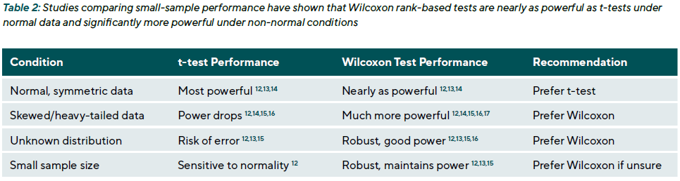
Non-parametric methods are also advantageous in small-sample studies. When the sample size is small (e.g., < 25 per group), assumptions about the distribution are harder to verify. Studies comparing small-sample performance have shown that Wilcoxon rank-based tests are nearly as powerful as t-tests under normal conditions and significantly more powerful under non-normal conditions (Table 2).
While parametric tests are powerful and efficient under ideal conditions, non-parametric methods offer robustness, flexibility, and practical advantages in the complex and often imperfect reality of clinical eye research. Understanding their respective assumptions and trade-offs enables researchers to select the most suitable test for their data, thereby enhancing the reliability and validity of their research findings.
A practical framework for choosing between parametric and non-parametric tests
The selection of an appropriate statistical test should be grounded in the outcome‘s measurement level, the data distribution characteristics, sample size, and the study‘s tolerance for error types. The following steps offer a structured approach for test selection:
- Consider the measurement level: If the outcome variable is nominal (categorical) or ordinal, parametric tests such as t-tests or ANOVA are not valid. Instead, non-parametric or categorical data methods should be used. For example, glaucoma severity grades on an ordinal scale should be analysed using a Mann-Whitney U test or, if treated categorically, a chi-square test, not a t-test.
- Assess distribution and sample size: For continuous outcomes, examine the distribution using histograms, Q-Q plots, or normality tests (e.g. Shapiro-Wilk). The sample size also affects test choice. For large samples, the Central Limit Theorem 4 implies that the ampling distribution of the mean approaches normality, even if the raw data are non-normal. For example, the mean axial length in a
sample of 2000 eyes may not be normally distributed, but a t-test could still be valid. In smaller samples, greater attention should be paid to distribution shape and the presence of outliers. - Check for outliers and skewness: Outliers can be detected using boxplots, z-scores, or robust statistics. These should be evaluated clinically to determine whether they are valid values or potential data errors. In eye research, outliers may reflect biological variability, such as extreme tear osmolarity in severe dry eyes. Similarly, skewness should be assessed visually and quantitatively. Both conditions can undermine the validity of parametric tests.
- Attempt data transformation, if appropriate: When data are non-normal but continuous, transformation may enable the use of parametric methods. Common transformations include:
- Logarithmic (e.g. for endothelial cell counts, cytokine levels)
- Square root or reciprocal (for count-type or right-skewed data)
- logMAR transformation, a standard in vision science, which converts non-linear Snellen visual acuity scores into an interval-scaled, approximately normal distribution
If the transformed data meets assumptions, a parametric test may be applied. Interpretation should be on the transformed scale, or results should be back-transformed for reporting.
- Use non-parametric methods when assumptions cannot be met: If the data remains non-normal after transformation or if the outcome is ordinal, a non-parametric test is more appropriate. For instance, in pre-post comparisons of central corneal thickness with heavily skewed values (e.g. due to advanced ectasia), the Wilcoxon signed-rank test should be preferred over the paired t-test.
- Weigh the consequences of type I and type II errors: The relative importance of avoiding false positives vs. false negatives should inform test selection. If the goal is to detect subtle effects (e.g. in exploratory studies), and the assumptions are marginally met, a parametric test may be acceptable to maximise power. Conversely, if the consequence of a false positive is high, such as in safety endpoints, a more conservative approach using non-parametric or permutation tests may be warranted.
- Report and justify the choice transparently: Clearly state the rationale for test selection, especially when a non-parametric method is used. For example: “Because macular pigment optical density was right-skewed and remained non-normal after log transformation, a non-parametric Mann-Whitney U test was used for group comparisons.” Reporting both the median with interquartilerange (IQR) and the mean with standard deviation can be useful, provided it is clear which summary measure aligns with the inferential test that was applied.
Transparency in reporting improves the interpretability and credibility of findings. It is often useful to report both the median with interquartile range (IQR) and the mean with standard deviation, as long as it is clear which summary aligns with the inferential test applied.
Common statistical tests in eye and Vision Research: Applications and examples
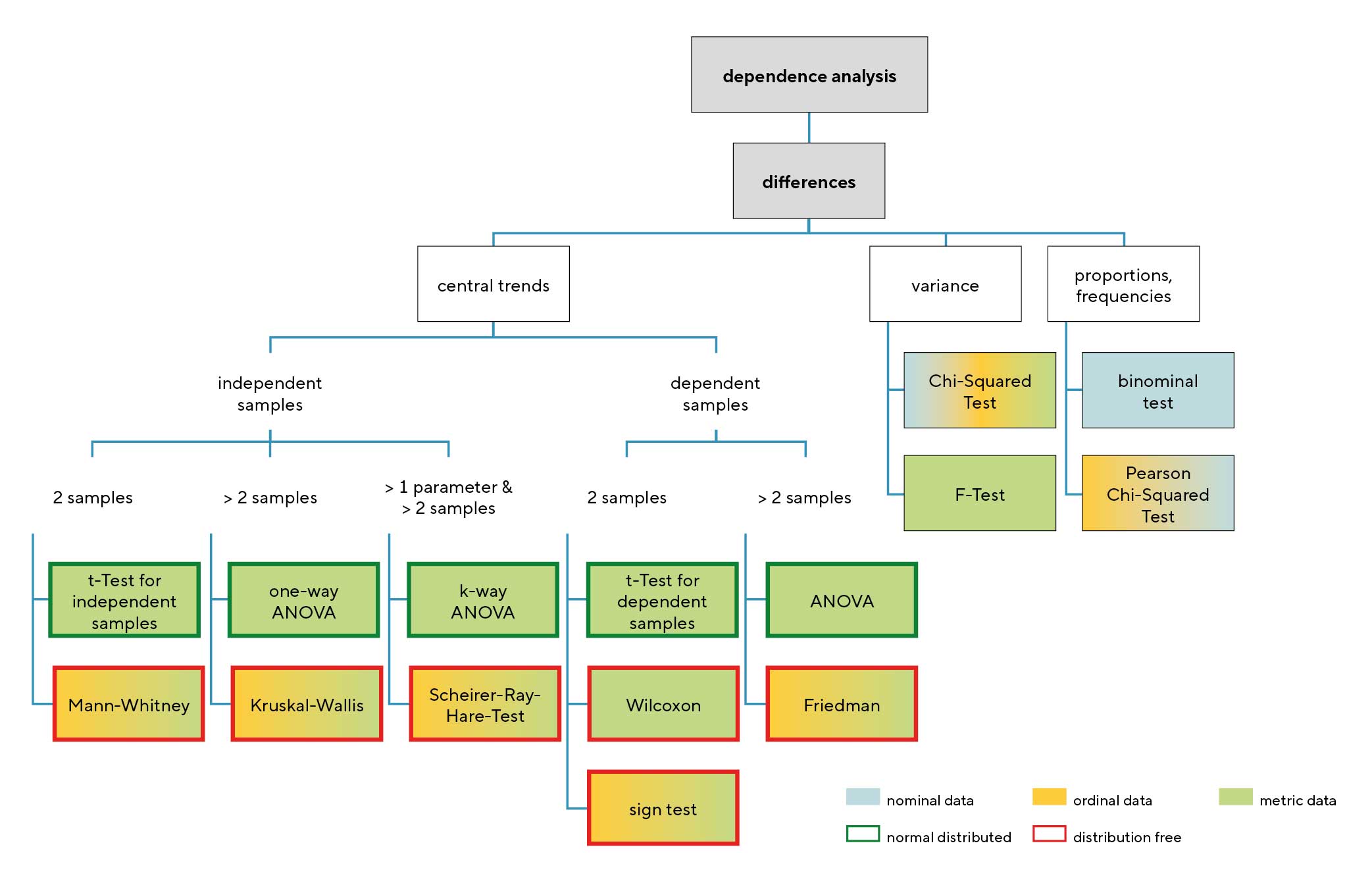
This chapter details several common statistical tests used in eye and vision research. The selection of an appropriate test is a critical step in data analysis, guided by the research question, study design, and the nature of the data. Figure 2 provides a flowchart that visually maps out this decision-making process, categorising tests based on the type of comparison, the number and independence of the samples, and the data‘s characteristics.
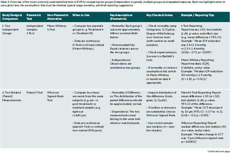
Comparing two independent groups:
t-Test and Mann-Whitney U Test
When an outcome is measured in two independent groups, such as patients receiving different treatments or fellow eyes from separate individuals, the appropriate statistical approach depends on the data’s measurement scale and distributional characteristics.
Independent Samples t-Test: The independent samples t-test, also known as the two-sample t-test, compares the means of a continuous variable between two unrelated groups. This test assumes that the outcome variable is approximately normally distributed within each group, that variances are equal (homoscedasticity), and that observations are independent. The t-test is a powerful and efficient method
if these conditions are met.
Clinical example 4: In a clinical trial, 40 patients with glaucoma are randomised to receive either Medication X (n = 20) or Medication Y (n = 20). After one month, the mean ± SD change in IOP was 3.8 ± 1.5 mmHg for Medication X vs. 2.5 ± 1.4 mmHg for Medication Y. The data in both groups were approximately normally distributed. An independent samples t-test was used to compare the means.
Mann-Whitney-U-Test: The Mann-Whitney U test (also known as the Wilcoxon rank-sum test) is the non-parametric alternative to the t-test. It is appropriate when the data are ordinal, non-normally distributed, or contain outliers that violate parametric assumptions. Rather than comparing means, this test evaluates whether one group tends to have higher values than the other based on ranks. It is often applied to outcomes like visual analogue scale ratings for discomfort or to continuous variables with skewed distributions.
Clinical example 4 (continued): If, in the same IOP example, the data were not normally distributed (e.g., due to a subgroup of non-responders creating a skewed distribution), a Mann-Whitney U test would be the correct choice. The test would rank all 40 IOP changes from smallest to largest and compare the sum of ranks between the two groups. A result of U = 130 with p = 0.012 would indicate a statistically significant difference, suggesting that patients receiving Medication X generally experienced greater IOP reductions than those on Medication Y.
Reporting tip: When reporting a t-test result in a journal, results should be reported as: “The mean ± SD change in IOP was 3.8 ± 1.5 mmHg for Medication X vs 2.5 ± 1.4 mmHg for Medication Y. This difference was statistically significant (two-sample t-test: t(38) = 2.75, p = 0.009).” For a Mann-Whitney, since medians are often reported: “The median IOP reduction was 4.0 mmHg (IQR 2.5 to 5.0) with X and 2.5 mmHg (IQR 1.5 to 3.5) with Y (Mann-Whitney U = 130, p = 0.012).”
It’s also good practice to mention that the test was two-tailed and to confirm distributional decisions (e.g., “due to a non-normal distribution, a non-parametric test was used”).
Comparing two paired measurements:
paired t-test and Wilcoxon signed-rank test
Paired data arise frequently in EVR. Typical examples include pre- and post-treatment measurements from the same Patient (e.g. visual acuity before and after cataract surgery) or comparisons between two eyes of the same individual, where one eye receives treatment, and the fellow eye serves as a control. In such cases, observations are not Independent and must be analysed using methods that account for within-subject correlation.
Paired t-test: The paired t-test is the parametric method for comparing two related measurements. Rather than comparing group means directly, the test calculates the difference between paired observations and assesses whether the mean difference significantly differs from zero. The key assumption is that the distribution of these difference scores (not the raw data) is approximately normal. When this condition is met, the test is efficient and widely used.
Clinical example 5: In a study of corneal collagen cross-linking, central corneal thickness (CCT) was measured before and six months after surgery in 15 treated eyes. The mean preoperative CCT was 520 μm (SD = 30), and the postoperative mean was 510 μm (SD = 32), yielding a mean change of –10 μm. If the distribution of these differences appears symmetric, a paired t-test can be applied. A result of t(14) = –5.0, p < 0.001, indicates a statistically significant thinning of the cornea post-treatment. The interpretation would be that CCT decreased on average by 10 μm (95 % CI: –13.7 to –6.3 μm).
Wilcoxon Signed-Rank Test: When the assumptions of the paired t-test are not met, for instance, if the distribution of differences is skewed or contains outliers, the Wilcoxon signedrank test provides a robust non-parametric alternative. This test ranks the absolute values of the paired differences and evaluates whether the changes are systematically positive or negative. No assumption of normality is required.
Clinical example 5 (continued): In the same dataset, if several eyes show little change while others show marked thinning or thickening, the distribution of differences may be skewed. Applying the Wilcoxon signed-rank test in this scenario might yield p = 0.0005, similarly indicating a significant postoperative decrease in CCT. The median change could then be reported as –9 μm, highlighting a robust central tendency despite the skewed distribution.
A crucial point on study design: It is essential to identify paired designs correctly. The sample size in a paired Analysis is the number of pairs, not the total number of measurements. In the example above, n = 15 pairs, not 30 measurements. Misapplying an unpaired test to paired data incorrectly inflates the sample size and can lead to erroneously small p-values. Conversely, applying a paired test to unpaired data is statistically invalid.
Comparing multiple independent groups:
ANOVA and Kruskal-Wallis Test
In many clinical studies, comparisons are required across more than two independent groups. For example, refractive error may be compared across age groups, or postoperative outcomes may be evaluated among patients receiving different surgical techniques. In such cases, the use of multiple t-tests introduces a high risk of Type I error due to repeated comparisons. To avoid this, Analysis of Variance (ANOVA) is used as the standard parametric method for comparing means across three or more groups.
One-Way ANOVA: One-way ANOVA tests the null hypothesis that all group means are equal. It compares between- group variability to within-group variability to determine whether group membership is associated with a statistically significant difference in the outcome. The assumptions include approximate normality of the Outcome variable within each group, homogeneity of variances, and independence of observations. The method is relatively robust to modest violations of variance equality if sample sizes are balanced.
When ANOVA yields a significant result (e.g., p < 0.05), it indicates that at least one group mean differs significantly. However, it does not specify where the difference lies. Posthoc comparisons, such as Tukey’s Honest Significant Difference (HSD) or Bonferroni-adjusted pairwise t-tests, are then used to identify which group pairs differ while controlling for multiple comparisons.
ANOVA can be extended to more complex designs, such as two-way ANOVA, to evaluate interactions between multiple factors (e.g. lens material × wear time in a 3 × 2 factorial design). Non-parametric alternatives for factorial designs are less well-established. In practice, researchers often attempt data transformation to permit parametric analysis or adopt custom rank-based methods where available.
Clinical example 6: A study compares comfort ratings (on a 0 – 100 scale) for three contact lens materials: hydrogel, silicone hydrogel, and a novel water-gradient material (n = 30 per group). A one-way ANOVA yields F(2,87) = 6.4, p = 0.003, indicating a significant difference among the materials. Posthoc Tukey testing then reveals that the water-gradient lenses are rated significantly more comfortable than both Hydrogel (p = 0.002) and silicone hydrogel (p = 0.04), while the difference between hydrogel and silicone hydrogel is not significant (p = 0.10).
Kruskal-Wallis Test: When data are not normally distributed or are ordinal, the Kruskal-Wallis test serves as the non-parametric alternative to one-way ANOVA. It tests whether at least one group differs in distribution by ranking all observations and comparing mean ranks. The null hypothesis is that all groups are drawn from the same distribution. If p < 0.05, post-hoc pairwise comparisons (e.g. Mann-Whitney U tests
with Bonferroni correction) can identify which groups differ.
Clinical example 6 (continued): If the lens comfort data were skewed, a Kruskal-Wallis test would be used. A result of χ²(2) = 9.5, p = 0.009 would indicate significant differences. Subsequent pairwise Mann-Whitney tests with a Bonferroni- adjusted α = 0.017 might show that the water-gradient lens is significantly more comfortable than the hydrogel lens (e.g., p = 0.003), while other comparisons do not reach the corrected significance threshold.
Reporting tip: When reporting an ANOVA result, include group means, standard deviations, the test statistic with Degrees of freedom, and the p-value. For example: “The mean ± SD comfort scores were 75 ± 10 for hydrogel lenses, 80 ± 8 for silicone hydrogel, and 85 ± 5 for water-gradient lenses. One-way ANOVA showed a statistically significant difference in mean comfort scores across materials (F(2,87) = 6.4, p = 0.003). Post-hoc Tukey tests indicated that water-gradient lenses were rated significantly more comfortable than Hydrogel (mean difference = 10, p = 0.002) and silicone Hydrogel lenses (mean difference = 5, p = 0.04).”
When reporting a Kruskal-Wallis result, median and IQR values are typically provided, along with the chi-square statistic and p-value. For example: “The median comfort scores were 74 (IQR 68–80) for hydrogel, 79 (IQR 75–85) for Silicone hydrogel, and 86 (IQR 82–90) for water-gradient lenses. The Kruskal-Wallis test indicated a significant difference among groups (χ²(2) = 9.5, p = 0.009). Post-hoc Mann-Whitney U tests with Bonferroni correction showed that comfort was significantly higher with water-gradient lenses compared to hydrogel (U = 250, p = 0.003), but the difference between water-gradient and silicone hydrogel lenses did not reach the corrected significance threshold (U = 320, p = 0.02; α = 0.017).”
Always clarify why a non-parametric method was chosen if applicable, for example: “Due to skewed distributions and ordinal scaling of comfort scores, a non-parametric test was used.”
Repeated measures and longitudinal data:
Repeated-Measures ANOVA and Friedman Test
In EVR, it is common for outcomes to be measured multiple times within the same individuals, across time points, conditions, or interventions. This within-subject or repeated-measures design allows each subject to act as their own control, thereby reducing between-subject variability and increasing statistical power. However, standard ANOVA Independence assumptions are violated because repeated measurements on the same individuals are correlated.
Repeated-measures ANOVA extends the one-way ANOVA framework to account for within-subject correlation. It is used when a continuous outcome is measured at multiple time points or under different conditions for the same subjects and when the assumptions of approximate normality and sphericity (equal variances of the differences between all pairs of conditions) are met. When the sphericity assumption is violated, corrections such as Greenhouse-Geisser or Huynh-Feldt are applied to adjust degrees of freedom and p-values.
Clinical example 7: In a study of postoperative visual recovery, best-corrected visual acuity (BCVA, logMAR) is measured in 10 patients at 1 week, 1 month, and 3 months after cataract surgery. A repeated-measures ANOVA Tests whether mean logMAR changes significantly over time. An analysis yielding F(2,18) = 5.5, p = 0.013, suggests a significant difference across time points. Post-hoc comparisons (e.g., paired t-tests with Bonferroni correction) might then Show that significant improvement occurred between 1 week and 1 month (p < 0.01), but not between 1 month and 3 months (p = 0.314).
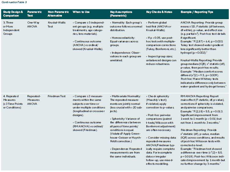
Friedman Test: When the assumptions for repeated-measures ANOVA are not satisfied, particularly in small samples or with ordinal or skewed data, the Friedman test offers a non-parametric alternative. It ranks the measurements within each subject and tests whether the average rank differs across conditions. The test evaluates whether at least one condition systematically differs in distribution without assuming normality or sphericity.
Clinical example 7 (continued): If the logMAR values in the above study were not normally distributed, the Friedman test would be more appropriate. A result of χ²(2) = 8.0, p = 0.018 would again indicate a statistically significant change over time. Post-hoc pairwise Wilcoxon signed-rank tests could then be used to identify where the specific differences occurred.
A note on missing data: Both repeated-measures ANOVA and the Friedman test typically require complete data for each subject across all measurement points. Missing data from missed visits or incomplete assessments must be handled carefully, either by excluding those cases (if few) or by using more advanced methods like mixed-effects models, which can account for missing data and are beyond the scope of this article.
Each of these tests helps guard against the play of Chance by providing a p-value to inform decisions about the hypotheses. However, a p-value alone is not enough; the size of the effect and confidence intervals also need to be considered to understand what the data are telling.
Interpreting statistical significance: p-values, confidence intervals, and effect sizes
When reporting the results of statistical tests, Researchers often focus on the p-value and whether it exceeds the conventional threshold of 0.05. However, reliance on “p < 0.05” alone has been widely criticised for oversimplifying results.18,19,20,21 A finding can be statistically significant yet clinically trivial, or vice versa. To interpret results responsibly, especially in a clinical field, one must look beyond the p-value to confidence intervals and effect sizes.
The p-Value revisited: A p-value is often misunderstood. It is not the probability that the null hypothesis is true, nor the probability that the observed effect was due to chance in the sense of a real vs chance cause. Rather, as defined earlier, it’s the probability of obtaining the observed data (or something more extreme) if the null hypothesis were true. For example, p = 0.03 in a trial of an anti-VEGF drug for macular oedema means: “If the drug had no real effect, there’s a 3 % Chance we’d see an improvement as large as observed.” It does not mean “there’s a 97 % chance the drug works”. Many experienced researchers mistakenly interpret p this way. P-values do not measure the probability that H₀ is true or that data were produced by random chance alone.
Scientific conclusions should not be based only on whether the p-value passes a threshold (e.g. 0.05). In other words,treating 0.049 as a success and 0.051 as a failure is an arbitrary dichotomy and can be misleading. Small changes in data or analysis can shift a result from significant to non-significant without fundamentally altering the clinical message.
One issue is the sample size: some studies have small sample sizes due to difficulties in recruiting participants (rare diseases, invasive procedures, etc.), leading to p-values that might be greater than 0.05 even if there is a moderate effect (risk of Type II error). Conversely, large datasets (e.g. big epidemiological studies or large trials) can produce Tiny p-values for very small statistically “real” differences but
clinically negligible. Both scenarios require judgment beyond the p-threshold.
Confidence Intervals (CIs): A CI gives a range where the true effect likely lies. A 95 % CI means that, over many repetitions, 95 % of such intervals would contain the true value. For example, if a treatment improves contrast sensitivity by 0.10 log units with a 95 % CI of 0.02 to 0.18, the true effect could range from 0.02 to 0.18. If the interval excludes 0, the result is statistically significant at the 0.05 level. CIs reflect both precision and effect size. Clinical relevance depends not just on whether an effect exists (p-value) but on whether it‘s large enough to matter. For this reason, many journals now require CIs alongside p-values.
Clinical example 7: Consider an RCT comparing two glaucoma drops: mean IOP reduction differs by 1.0 mmHg (p = 0.04), with a 95 % CI of 0.1 to 1.9 mmHg. Though “significant,” the clinical importance is debatable, some specialists consider 20 % change mmHg necessary to justify changing therapy.22,23,24 Conversely, a non-significant result with a wide CI, e.g. 1 mmHg difference, p = 0.2, CI –0.6 to +2.6, shows uncertainty. The effect could be meaningful or null, suggesting limited power. Reporting “no significant difference” without noting this uncertainty is misleading.
Effect sizes: CI show the plausible range for an effect, while effect size metrics quantify how large that effect is in a standardised way. For comparing means, for instance, Cohen’s d expresses the mean difference in units of the pooled Standard deviation.25
Clinical example 8: If treatment A improves visual acuity by 0.1 logMAR more than treatment B, and the pooled SD is 0.2 logMAR, the effect size is Cohen‘s d =x0.5, which is considered a medium effect. If the pooled SD were only 0.05 logMAR, the effect size would be d = 2.0, a very large effect.
Effect sizes like Cohen‘s d, odds ratios (for binary outcomes), or η² (for ANOVA) are vital because statistical significance alone does not indicate clinical importance. Small, clinically trivial effects can be highly significant in large studies, while large, potentially important effects may not reach statistical significance in small studies.
In eye care, established clinically meaningful benchmarks help interpret results, such as a change of 0.1 logMAR (5 ETDRS letters) in visual acuity or 1 dB in visual field mean deviation. Effects smaller than these may be clinically unimportant even if p < 0.05; conversely, larger effects may Warrant attention even if p > 0.05.
Given the known limitations of relying solely on p-values, clinical relevance is often best captured by the Minimum Clinically Important Difference (MCID).26 The MCID represents the smallest change in an outcome that a patient would perceive as beneficial or that would prompt a change in their clinical management. Ideally, clinical trials should be designed with sufficient power to detect an effect at least as large as the MCID, and the results should be interpreted in this context.
To ensure robust conclusions, researchers should be aware of several common pitfalls when interpreting statistical results.
- Dichotomous Thinking („p = 0.049 vs p = 0.051“): Treating results as a simple „success“ or „failure“ based on the 0.05 threshold leads to dichotomous thinking. Instead of using ambiguous phrases like „trended towards significance,“ it is better to report the exact p-value and confidence interval. This allows the reader to assess the evidence,especially when the effect size is substantial but the result narrowly misses the significance threshold.
- Multiple Comparisons and p-Hacking: When many Outcomes or analyses are performed, the chance of obtaining a small p-value increases by chance alone. This can lead to reporting spurious findings. As discussed later, Adjustments for multiple comparisons are often necessary to control this risk.
- Non-significant results do not indicate the absence of an effect: It is a common mistake to conclude „there was noeffect“ when p > 0.05. The correct interpretation is that „no statistically significant effect was found.“ The confidence interval is crucial here: does it rule out a clinically meaningful effect, or is it very wide, suggesting the study was inconclusive (i.e., underpowered)? For example: “We did not find a significant difference in retinal nerve fibre layer thickness between groups (mean difference 2 μm, 95 % CI –3 to +7, p = 0.4), suggesting any true difference is likely small.”
- Over-reliance on „Significant“ Labels: A „statistically significant“ result is not automatically an important one. In large observational studies, very small, clinically trivial differences can produce tiny p-values. Always circle back to the effect size and its clinical relevance to judge the practical importance of the finding.
Clinical relevance: In evidence-based practice, both the presence and size of effects matter. A treatment might significantly alter an imaging parameter but offer no perceptible benefit to patients, limiting its value. Conversely, a large Risk reduction in blindness from a pilot study (p = 0.1) may still warrant attention if the effect is clinically important but the sample is small.
p-values help assess whether findings are likely due to chance but must be interpreted in context. CIs show theplausible range of the effect and whether it crosses clinically relevant thresholds. Effect sizes quantify Magnitude in a standardised way. Ophthalmic research should report all three, p-values, CIs, and effect sizes, to ensure statistical results are clinically meaningful. This approach prevents Overstatement or neglect of findings and better aligns statistical analysis with clinical judgment.
Reporting tip: When presenting results, include the effect size and its confidence interval, not just the p-value. For example: “Treatment A reduced IOP by 1.2 mmHg more than Treatment B (95 % CI: 0.3 to 2.1 mmHg; p = 0.01; Cohen’s d = 0.6).” This allows readers to judge both significance and clinical relevance. Always specify the test used, whether it was two-tailed, and justify any distributional assumptions (e.g. use of non-parametric methods for skewed data).
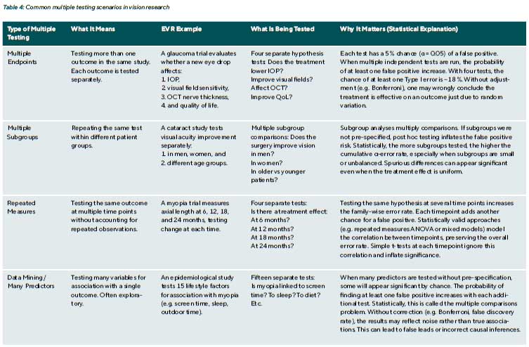
Multiple comparisons and adjustments: Controlling false positives
Modern studies often measure numerous outcomes. A clinical trial for glaucoma might assess IOP, visual field indices, optic nerve imaging metrics, and quality of life, multiple endpoints. Similarly, an observational study may examine multiple predictors for their association with a disease outcome.
The problem of multiple testing
Multiple testing is a common statistical issue in EVR (Table 4). Each time a hypothesis test is performed, there is a chance(α) of a false positive. When multiple tests are done, the possibility of at least one false positive increases. Multiple comparisons (or multiple testing) are a critical issue: without correction, one might be misled by apparently significant findings that are merely random noise. For example, testing
20 independent outcomes at α = 0.05, on average, one will be significant by chance alone.
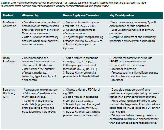
Adjustment techniques
Multiple comparison adjustments reduce false positives (Type I errors) when many tests are performed. Common goals include controlling the Family-Wise Error Rate (FWER), which is the probability of at least one false positive, and the False Discovery Rate (FDR), which is the proportion of false positives among significant results (Table 5).
Clinical example 9: Multiple endpoints in a dry eye trial A study of a new dry eye therapy evaluates four outcomes: (1) Symptom score (2) Tear Break-Up Time (TBUT) (3) Corneal staining grade (4) Schirmer test. Each is tested at α = 0.05.
The p-values are:
- Symptoms: 0.01 (significant)
- TBUT: 0.04 (significant)
- Staining: 0.20 (not significant)
- Schirmer: 0.03 (significant)
Conclusion: Without correction, researchers might claim the treatment significantly improved symptoms, TBUT, and Schirmer results.
Bonferroni Correction:
- Adjust α for four tests: α = 0.05 / 4 = 0.0125
- Only Symptoms (p = 0.01) remain significant
- TBUT (0.04) and Schirmer (0.03) > 0.0125 → not significant
Conclusion: Only symptom improvement is statistically robust. Other effects may be trends but are not conclusive.
Holm–Bonferroni Method:
- Order p-values: 0.01, 0.03, 0.04, 0.20
- Compare each to adjusted thresholds:
< 0.05/4 = 0.0125 → significant
< 0.05/3 ≈ 0.0167 → not significant - Holm stops at the first non-significant test.
Conclusion: Only symptoms pass. TBUT and Schirmer are not significant.
Benjamini–Hochberg (FDR 5 %):
- Sorted p-values: 0.01, 0.03, 0.04, 0.20
- Compare each to (i/4) × 0.05:
< 0.0125 (i = 1) → yes
> 0.025 (i = 2) → no → stop
Conclusion: Only symptoms meet the FDR threshold.
Interpretation: All three methods agree: only the symptom improvement is statistically reliable. TBUT and Schirmer do not reach significance after correcting for multiple comparisons. If these outcomes are highly correlated (e.g. symptom scores improve with TBUT), Bonferroni may be overly strict. In such cases, alternative methods like Hochberg’s step-up or no correction may be considered, but only if co-primary outcomes were pre-specified with a strong clinical rationale. Corrections are most important when testing many outcomes
without prior justification.
Clinical example 10: Multiple arms in a surgical trial
A study compares three surgical techniques (A, B, C) for correcting refractive error.
Outcomes include:
- Post-operative refraction
- Uncorrected distance visual acuity (UDVA)
Step 1: Initial comparison – One-Way ANOVA
Researchers run a one-way ANOVA on post-op refraction to test whether there is any overall difference among the three groups.
Result: ANOVA p = 0.02 → suggests at least one group differs significantly in mean refraction.
Conclusion: ANOVA tells you a difference exists, but not which groups differ.
Step 2: Post-Hoc Testing – Which groups differ?
There are three possible pairwise comparisons: (i) A vs B (ii) A vs C (iii) B vs C
Option A: Correct Approach – Tukey’s HSD or Dunnett’s Test:
These are post-hoc methods designed to control for multiple comparisons:
- Tukey‘s HSD compares all group pairs and keeps the Family-Wise Error Rate (FWER) at 0.05.
- Dunnett‘s test compares each group to a control Group (e.g. A vs B, A vs C), also controlling FWER.
Without adjustment, running multiple pairwise tests increase the risk of false positives. For 3 comparisons at α = 0.05 each, the chance of at least one false positive is ~14% (1 – 0.95³).
Option B: Incorrect Approach – Three Unadjusted t-tests:
If a researcher ran three independent t-tests at α = 0.05:
A vs B: p = 0.04
A vs C: p = 0.03
B vs C: p = 0.08
They might conclude that A differs from B and C. But this approach inflates the Type I error rate because each test is treated in isolation. Even if no real difference exists, one test could appear significant by chance.
Conclusion: Correct interpretation with Tukey’s test: Only report pairwise differences if they remain significant after Tukey adjustment. Tukey accounts for the number of comparisons, so p-values are slightly higher, but false positives are controlled.
Step 3: Interpretation and conclusion
The ANOVA shows there is a difference in refraction between at least two surgical groups. The Tukey test identifies which specific pairs differ, while keeping the error rate under control. If only A vs C is significant after adjustment, the conclusion is: “Surgical method A resulted in significantly different post-op refraction compared to C (p = 0.03, Tukey-adjusted), with no significant differences between A and B or B and C.”
There is ongoing debate about whether adjustment for multiple comparisons is necessary when outcomes are pre-specified and reflect distinct aspects of the study’s objectives. Some argue that outcomes may be reported individually with appropriate caution if they are clinically meaningful and independent.27,28,29 However, the standard practice clearly distinguishes primary from secondary outcomes and applies the strictest statistical threshold to the primary endpoint. In contrast, adjustments are generally recommended for subgroup analyses and exploratory outcomes; at the very least, such findings should be explicitly labelled as exploratory and interpreted as hypothesis-generating rather than confirmatory.
A common approach in practice is to predefine a single primary outcome tested at α = 0.05, with other outcomes treated as secondary, either reported descriptively or requiring confirmation in future studies. CONSORT guidelines 30 recommend specifying which outcomes are primary and whether adjustments for multiple comparisons were made. When multiple tests are performed without adjustment, authors should disclose this and interpret it cautiously. For example, a secondary outcome with p = 0.03 may be described as “nominally significant, unadjusted for multiple comparisons.”
Reporting tip: Authors should clearly state whether Adjustments for multiple comparisons were applied and specify the method used. For example:
- “A Bonferroni correction was applied for the three Primary comparisons, setting the threshold for significance at p < 0.017.”
- “All pairwise post hoc comparisons were adjusted using Tukey’s method to control the family-wise error rate.”
- “Given the number of secondary endpoints, results are interpreted descriptively. For instance, tear cytokine Levels differed nominally between groups (p = 0.03) but did not meet the adjusted significance threshold (p < 0.01).”
Transparent reporting ensures appropriate interpretation of results and guards against overstating findings due to inflated Type I error.
Balancing Type I and Type II errors: Adjusting for multiple comparisons reduces the risk of false positives (Type I errors) but increases the risk of false negatives (Type II errors), potentially obscuring true effects. For example, if a Treatment genuinely influences several related outcomes, a strict correction, such as the Bonferroni method, may make it harder to detect those effects. In such cases, researchers may consider using composite outcomes or multivariate methods (e.g. MANOVA) to assess an overall effect across endpoints. While these approaches are beyond the current scope, the key principle remains: the more tests performed, the more cautious one must be in interpreting individual p-values.
Transparent reporting and best practices
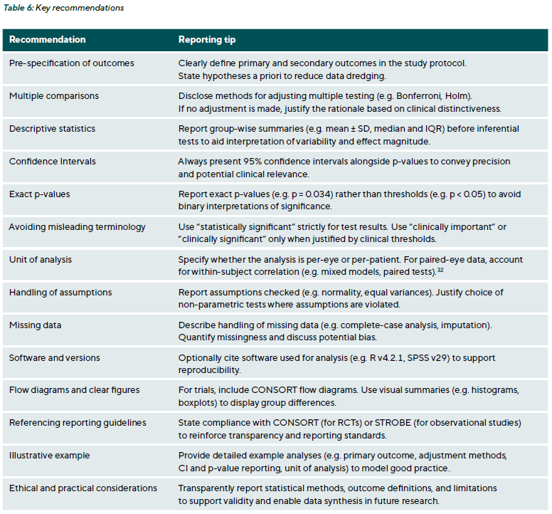
Robust study design and appropriate statistical analysis contribute little to EVR if the results are not reported transparently. Clear communication of methods and findings helps readers evaluate how conclusions were reached and whether they apply in clinical contexts. Two cornerstone guidelines (1) CONSORT 30 (Consolidated Standards of Reporting Trials) for randomised controlled trials and (2) STROBE 31 Strengthening the Reporting of Observational Studies in Epidemiology) for observational studies, call for detailed accounts of statistical procedures. For example, CONSORT item 12 requires specifying “statistical methods used to compare groups for primary and secondary outcomes,” while STROBE requests explanations of how missing data were handled and whether sample size calculations were performed. To find the most appropriate validated reporting guidelines, refer to the EQUATOR network.
Beyond methodological rigour, transparent statistical reporting is an ethical imperative. In EVR, findings directly influence patient management; misreporting or selective presentation of data can lead to suboptimal decisions and tangible harm. Transparency helps patients benefit from genuine scientific progress rather than misleading claims. It also preserves the integrity of the scientific record by reducing research waste and supporting reproducibility. Researchers have a moral and professional obligation to report all outcomes, including non-significant or unfavourable ones, to avoid distorting the evidence base. Transparency fosters accountability, enabling peers to verify analyses and assess whether findings are robust enough to guide clinical practice. Adherence to ethical frameworks such as the Declaration of Helsinki (2024) and Good Clinical Practice, alongside reporting standards like CONSORT and STROBE, reinforces the duty to disseminate results responsibly and maintain public
trust in research.
Conclusion
Rigorous statistical testing constitutes a cornerstone of robust clinical decision-making in eye care. This article extends the foundational concepts of descriptive statistics (introduced in Part 1) by outlining core inferential principles and illustrating how Type I and Type II errors directly impact the validity of research outcomes. Clear guidance on parametric and non-parametric tests has demonstrated how data characteristics and study designs determine the most suitable analytic approach. Emphasising effect sizes and confidence intervals alongside p-values highlights the distinction between statistical significance and clinical relevance. Furthermore, the review of multiple-comparison procedures underscores the necessity of transparent reporting to prevent inflated error rates and misleading conclusions, particularly pertinent in ophthalmic studies with multiple endpoints. The practical examples and recommendations for reporting standards, such as STROBE and CONSORT, reinforce that sound statistical methodology and clear communication of results strengthen scientific rigour and foster evidence-based practice. Ultimately, by advancing statistical literacy within optometry and ophthalmology, patient care benefits from more reliable evidence, paving the way for improved treatment strategies and long-term outcomes.
Conflict of Interest:
The author declares that they have no affiliations with or involvement in any organisation or entity with any financial interest in the subject matter or materials discussed in this manuscript.
Funding Statement:
This article did not receive a specific grant from public, commercial, or not-for-profit funding agencies.
Contribution by the authors:
Daniela Oehring was the principal author and initiator of the article and was responsible for its conception, drafting, and writing.

About Daniela Oehring
Dr. - Faculty of Health, University of Plymouth, Plymouth, UK
Dr. Daniela Oehring ist Optometristin an der School of Health Professions an der University of Plymouth (UK).
COE Multiple Choice Questionnaire
The publication "Advancing Statistical Literacy in Eye Care: A Series for Enhanced Clinical Decision-Making" has been approved as a COE continuing education article by the German Quality Association for Optometric Services (GOL). The deadline to answer the questions is 1st September 2026. Only one answer per question is correct. Successful completion requires answering four of the six questions.
You can take the continuing education exam while logged in.
Users who are not yet logged in can register for ocl-online free of charge here.
in Glaucoma and Ocular Hypertension. Ophthalmol. Glaucoma, 5, 85-93.